The OPM and the Illiquidity Discount: Allocating Equity Value Across Common Shares, ADP and BSPCE
How to allocate equity value across common shares, preferred shares and BSPCE with the OPM.

Introduction: why a common share is never worth the total divided by the number of shares
An unlisted company raises funds from investors who subscribe preferred shares, opens a BSPCE plan for its employees, and then one day has to answer a seemingly simple question: what is a common share worth? The answer is almost never the result of naively dividing the total equity value by the number of shares outstanding, because preferred shares carry economic rights that common shares do not.
The Option Pricing Method (OPM) is the reference method, recognised by the American Institute of CPAs as well as by the International Valuation Standards Council, for allocating an already-known equity value across several classes of securities whose rights differ upon exit.
« Each class of securities can be viewed as an option on the total equity value, exercisable at different thresholds depending on the rank of its liquidation rights. », American Institute of CPAs, Accounting and Valuation Guide.
Three tensions converge in 2026 to make this topic more relevant than ever. First, the number of unlisted companies with at least two classes of securities keeps growing as successive financing rounds multiply. Second, setting the exercise price of BSPCE and employee stock option plans now requires a documented methodological justification, failing which the benefit granted can be requalified. Third, the four illiquidity discount models most cited in the literature, Chaffee, Longstaff, Finnerty and Ghaidarov, can produce results that vary by a factor of two for the same assumptions.
This article walks through, formula by formula, the complete mechanics of an OPM allocation: its definition, its academic origin, the four calculation methods used to implement it (Black-Scholes, Black-Scholes-Merton, the Cox-Ross-Rubinstein binomial tree and Monte Carlo simulation), the four illiquidity discount models that combine with it, and two fully worked cases on the same fictitious company at two distinct moments of its development.
Structure the valuation of your financial instruments with Hectelion
An allocation by share class, an illiquidity discount to document, or a BSPCE exercise price to justify: book a call with Hectelion to discuss your situation. Our team applies a multi-method methodology aligned with IVSC standards and market practice, with the French-Swiss double expertise that characterises our business valuation, startup valuation and financial instrument valuation mandates.
Acontos: get a free online estimate of your company's value
Before diving into the detail, Hectelion has developed Acontos, an online audit, due diligence and business valuation tool, powered by Claude Sonnet 5 by Anthropic and calibrated on Hectelion's methodology. From your financial statements, it produces a first estimate of the value of your shares within minutes, free of charge and without retaining any document. Launch the valuation simulator to get an order of magnitude, then keep reading to understand how it works.
Definition: what is the OPM?
The OPM (Option Pricing Method) is a method that models each class of securities of an unlisted company as a call option on the company's total equity value. It is not used to calculate that total value, but to allocate it across classes, common shares, preferred shares (or ADP), BSPCE and other dilutive instruments, according to their respective rights upon exit: liquidation rank, participating or non-participating preference, conversion thresholds.
The principle rests on a direct analogy with standard financial options. A non-participating preferred share with a 1.0x liquidation preference behaves, in terms of cash flows, exactly like the combination of a safe position up to a certain threshold and a call option beyond it: below the threshold, it receives a fixed amount; above it, it converts to common shares to capture the upside. Common shares and BSPCE, in turn, behave like call options whose strike price corresponds to the amount that must be exceeded before they start receiving any share of value.
This reading makes it possible to use the full toolkit of option pricing models, Black-Scholes first among them, to solve a problem that appears, at first glance, far removed from listed financial markets: how much is a common share of an unlisted startup worth once it has raised funds from investors benefiting from a liquidation preference. The OPM differs in this respect from the DCF method, which models discrete, probability-weighted exit scenarios (IPO, acquisition, liquidation) rather than a continuous distribution of future values.
Origin: from the Black-Scholes formula to the practice of allocation by share class
The option pricing formula bearing the names of Fischer Black and Myron Scholes was published in 1973 in the Journal of Political Economy, under the title « The Pricing of Options and Corporate Liabilities ». The same year, Robert Merton published an extension in the Bell Journal of Economics and Management Science incorporating a continuous dividend yield, giving rise to the so-called Black-Scholes-Merton (BSM) model. Merton and Scholes were awarded the Sveriges Riksbank Prize in Economic Sciences in 1997, Fischer Black having passed away in 1995.
The idea of applying this formula to allocate the equity of an unlisted company across share classes emerged later, carried by the American practice of so-called « 409A » valuations (named after the section of the Internal Revenue Code governing the setting of exercise prices for employee stock options). The American Institute of CPAs (AICPA) formalised the use of the OPM, the PWERM and the current value method as early as 2004, in an initial Practice Aid on equity securities issued as compensation; this document officially became an Accounting and Valuation Guide in its 2013 revision (updated in 2019), and remains the most cited methodological reference today.
In France, even though the BSPCE answers to its own tax framework codified in the General Tax Code, the underlying technical question, how to set a defensible exercise price for a dilutive instrument in a company with several share classes, is exactly the one the OPM solves. The International Valuation Standards Council has adopted a comparable logic in its IVS 200 standard (Business Valuation), §130.5 to 130.8, on complex capital structures.
Why use the OPM rather than a direct allocation
First, the exit horizon is uncertain. A company that has just raised funds generally knows neither when nor how it will be sold or listed: the OPM models this uncertainty through a continuous distribution of future values rather than an assumed imminent liquidation event.
Second, the company presents significant growth potential. A static allocation method, which would distribute the current value as if a liquidation were happening tomorrow, would ignore the probability that future value will far exceed the conversion thresholds of the preferences, and would therefore understate the share going to common stock and BSPCE.
Third, the capital structure includes several classes with interlocking rights. As soon as a liquidation preference, a conversion clause or an option pool coexist with common shares, a simple rule-of-three by share count becomes methodologically untenable.
Fourth, the objective is to set a defensible exercise price for BSPCE or employee stock options. An undervalued common share exposes the issuer to a real risk of tax requalification of the benefit granted; an overvalued one needlessly undermines the plan's attractiveness for beneficiaries.
Fifth, the auditability of the method matters as much as its result. The OPM rests on explicit, debatable and documented assumptions (volatility, horizon, risk-free rate), which makes it a robust method when reviewed by a statutory auditor, an auditor, or the tax authorities, unlike an arbitrary estimate.
How an OPM allocation by share class is built
Building an OPM allocation follows a six-step sequence, in this order, moving from the overall value to its fine-grained breakdown across classes.
Step 1, determine the total equity value. This value, denoted S0 in the formulas that follow, is obtained through the classic methods, discounted cash flow (DCF), trading and transaction market multiples, and adjusted net asset value (NAV), converging toward a single retained value. The OPM never replaces this step: it applies to its result.
Step 2, map the capital structure. Each class of securities must be listed, its number of shares, its liquidation rank, whether its preference is participating or not, and any fully diluted option pool or phantom instrument plan that could dilute the other classes.
Step 3, identify the breakpoints. A breakpoint is a total value level beyond which the economic behaviour of at least one class changes, typically the point at which a liquidation preference stops being advantageous relative to converting into common shares. Between two consecutive breakpoints, the rule for sharing additional value stays constant.
Step 4, choose the option parameters. Three assumptions drive the calculation: the expected volatility of the security (often estimated from listed comparables), the horizon T until the expected liquidity event, and the risk-free rate r matching that horizon.
Step 5, value each tranche as a call spread. The value of the tranche between two breakpoints K1 and K2 is obtained by taking the difference between the price of a call option with strike K1 and that of a call option with strike K2, both written on the same underlying value S0. The last tranche, beyond the final breakpoint, is simply worth the price of the call at that last strike.
Step 6, allocate each tranche to the classes concerned, then apply the discounts. Each tranche is split among the classes entitled to it, in proportion to their participation in that specific tranche. The resulting value per share is then, where applicable, reduced by an illiquidity discount (DLOM) specific to each class, covered in detail later in this article.
The four OPM calculation methods: formulas and variables
The four tranches described in step 5 above can be valued using four distinct methods, which all converge toward a very close result when assumptions are identical, but which differ in their flexibility and computational cost.
Black-Scholes (1973). For a non-dividend-paying stock, the price of a call option is written:
C = S·N(d1) − K·e−rT·N(d2)
d1 = [ln(S/K) + (r + σ²/2)·T] / (σ·√T) d2 = d1 − σ·√T
Each symbol corresponds to a precise input of the allocation:
- S: the total equity value as of the valuation date;
- K: the breakpoint under consideration, i.e. the threshold of the tranche being valued;
- r: the continuous risk-free rate matching horizon T;
- σ: the annualised volatility of S;
- T: the horizon, in years, until the expected liquidity event;
- N: the cumulative distribution function of the standard normal distribution, i.e. the probability that a standard normal variable is below the given argument.
Black-Scholes-Merton (1973 extension). When the underlying pays a continuous yield q, a dividend, or by extension a synthetic carry cost, the formula becomes:
C = S·e−qT·N(d1) − K·e−rT·N(d2)
d1 = [ln(S/K) + (r − q + σ²/2)·T] / (σ·√T)
The only new element compared with Black-Scholes is q:
- q: the continuous yield paid by the underlying over horizon T, zero for an unlisted company that pays no dividend (BSM then coincides exactly with Black-Scholes), or set to a positive synthetic value to represent the carry cost of holding an illiquid security for an extended period, an alternative to applying a full illiquidity discount downstream, discussed in the Limitations section below.
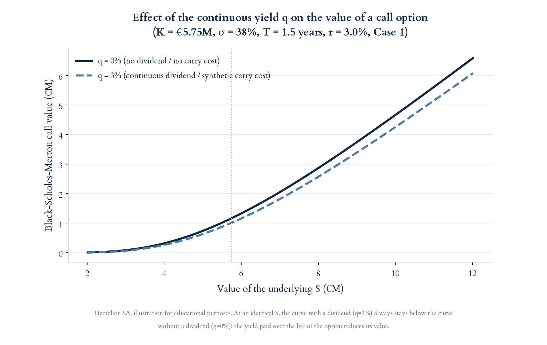
Reading the chart: for an identical underlying price S, the curve with a dividend (q = 3%) always stays strictly below the curve without a dividend (q = 0%), because part of the security's value is consumed by the yield paid over the life of the option, an effect that mechanically grows with the level of S.
Cox, Ross and Rubinstein binomial model (CRR, 1979). Published in the Journal of Financial Economics, this model discretises duration T into N intervals of length Δt = T/N, over which the underlying can move up or down:
u = eσ·√Δt d = 1/u p = (er·Δt − d) / (u − d)
The option value is then obtained through backward induction from the terminal payoffs:
- u: the up factor applied to the underlying at each step;
- d: the down factor, the exact inverse of u, which guarantees the tree recombines;
- p: the risk-neutral probability of an up move at each step, used to discount payoffs through backward induction, not the real-world probability of the security going up.
The model converges to Black-Scholes as N grows large, but retains the advantage of being able to handle irregular payoff structures or early exercise, which the closed-form formula cannot.
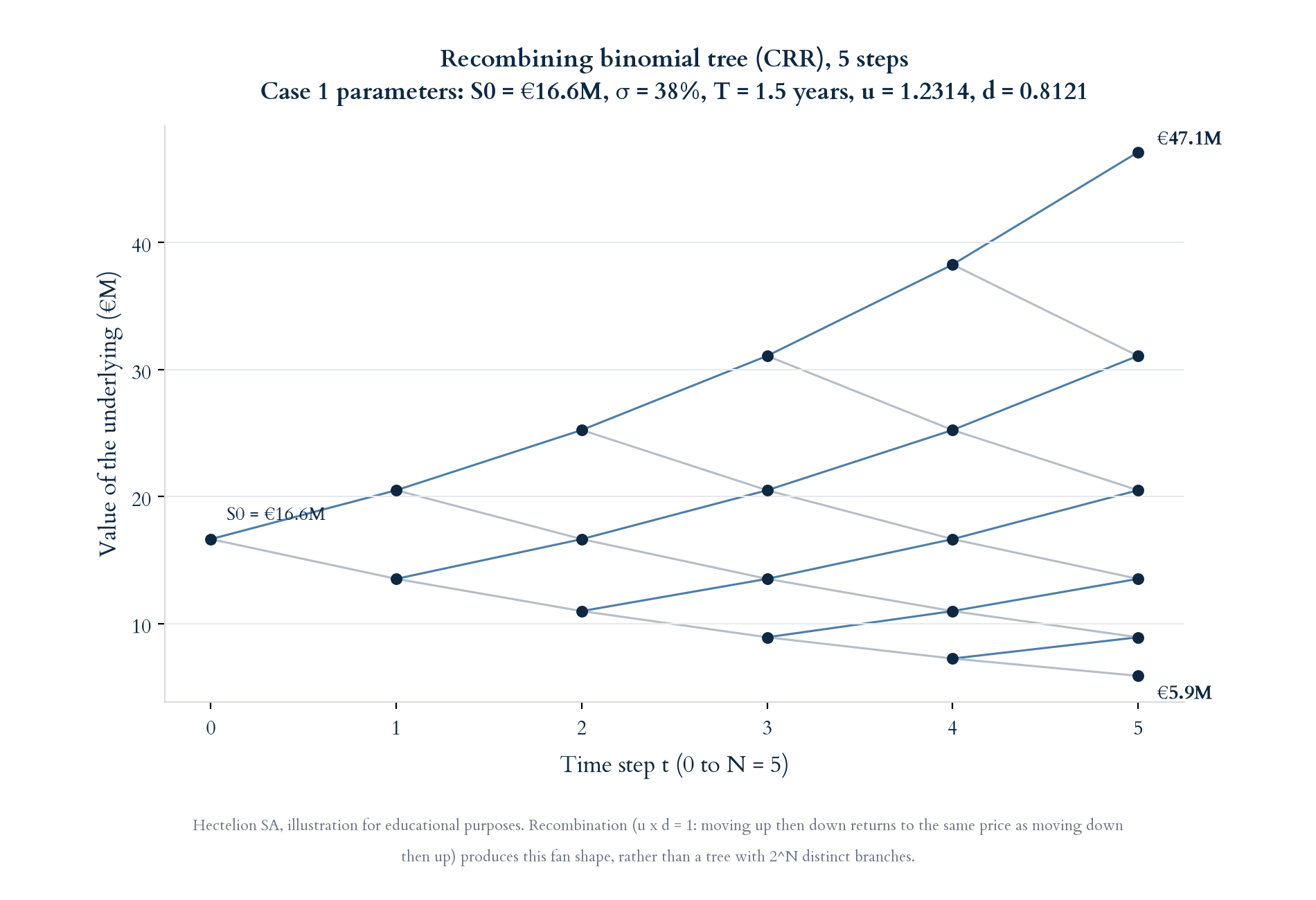
Reading the chart: it is the recombination of the tree, u multiplied by d equals exactly 1, that produces this fan shape rather than a line that only goes up or down: moving up then down brings you back to exactly the same price as moving down then up, so the number of distinct nodes at each step t grows only as t+1 rather than 2t. The calculation sheet in the « OPM CRR » tab of the downloadable Excel model at the end of this article mathematically builds this same recombining tree, each node depending only on the number of up moves rather than their order; this chart simply provides an intuitive visual representation of it.
Monte Carlo simulation. This method simulates a large number of random paths of the underlying:
ST = S0 · exp[(r − σ²/2)·T + σ·√T·Z]
where Z introduces the randomness of each path:
- ST: the simulated value of the underlying at horizon T on a given path;
- Z: a random variable drawn from a standard normal distribution, different for each simulated path.

Reading the chart: each thin blue line is an independent simulated path of S(t); the dispersion between paths visibly widens with time, in proportion to the square root of elapsed time, the direct signature of the security's volatility. It is precisely this diversity of simulated paths, not a closed-form formula, that gives the Monte Carlo estimate its value: the larger the number of paths, the more the discounted average of their payoffs converges to the theoretical price of the option.
On each of these paths, the exact payoff of the liquidation waterfall is computed security by security, then discounted at the risk-free rate and averaged across all paths. This is the most flexible method: only it can directly handle complex structures, capped participating preferences, multiple cascades, without having to artificially decompose them into vanilla options.
A note for the attentive reader: Hectelion has already published an article on valuing AI startups through growth real options, which uses exactly the same four mathematical tools, Black-Scholes-Merton, CRR and Monte Carlo included.
The two uses are not redundant, however, they answer two different questions with the same toolkit. In a growth real options framework, S represents the current value of an asset or a project, K the cost of a future investment, and T the horizon of the managerial decision to invest or not. In the context of this article, S represents the total, already-known, equity value of the company, K the breakpoints of the liquidation cascade across share classes, and T the horizon until the expected liquidity event. Same formula, entirely different object.
| Method | Principle | Short formula | Advantage | Limitation |
|---|---|---|---|---|
| Black-Scholes (1973) | Closed form, non-dividend stock | C = S·N(d1) − K·e-rT·N(d2) | Instant calculation, reference standard | Assumes constant volatility and rate over the whole period |
| Black-Scholes-Merton | Extension with continuous yield q | C = S·e-qT·N(d1) − K·e-rT·N(d2) | Can embed a synthetic carry cost | Double-counting risk if combined with a full DLOM |
| CRR, binomial tree (1979) | N-step discretisation, backward induction | u = eσ√Δt, p = (erΔt-d)/(u-d) | Handles early exercise and irregular payoffs | Heavier to compute, converges to Black-Scholes as N grows |
| Monte Carlo | Random path simulation | ST = S0·exp[(r-σ²/2)T+σ√T·Z] | Only method suited to complex, path-dependent waterfalls | Precision depends on the number of simulations, sampling noise |
Reading the table: the four methods are different computational paths toward the same economic quantity. Cases 1 and 2 below show, figures in hand, that they converge to within less than 0.1% between Black-Scholes and the CRR model, and to within less than 0.1% as well for the Monte Carlo simulation given residual sampling noise.
The four illiquidity discount (DLOM) models: authors, formulas and logic
Once the value of each class has been allocated through the OPM, an illiquidity discount (DLOM) must still be applied to securities that cannot be freely resold, typically the common shares and BSPCE of an unlisted company. The Discount for Lack of Marketability Job Aid published by the US Internal Revenue Service lists several families of models; four of them, grounded in option theory, dominate practice.
Chaffee (1993). David Chaffe models the discount as the cost of an at-the-money protective put option, hypothetically purchased to guarantee the resale of the security at its current price at the end of the restriction period:
DLOM = Put(S0, K=S0, r, σ, T) / S0
- Put(S0, K=S0, r, σ, T): the price of a European put option given by the Black-Scholes formula, with a strike K equal to the current price S0 (hence the at-the-money qualifier);
- S0: the security's value as of the valuation date, also used as the denominator to express the discount as a percentage.
Intuition: the higher the volatility and the horizon, the more expensive this insurance, and the larger the discount.
Longstaff (1995). Francis Longstaff, in the Journal of Finance, proposes a theoretical upper bound based on a lookback option: that of an omniscient investor who could have sold at the highest price observed throughout the restriction period. His simplified formula, often cited in practitioner literature, reads:
DLOM = 2·N(0.5·σ·√T) − 1
- σ: the annualised volatility of the security;
- T: the horizon, in years, of the restriction period;
- N: the cumulative distribution function of the standard normal distribution.
Because it assumes a perfect seller who never times the market wrong, this discount structurally constitutes a ceiling, rarely reached in practice, but useful as a reference bound.
Finnerty (2012). John Finnerty models the discount as the price of an average-strike Asian put option:
DLOM = E[max(S̄arith − ST, 0)] / S0
- S̄arith: the arithmetic average of the security's price observed over the entire restriction period;
- ST: the security's price at the end of that same period;
- E[...]: the expectation of this payoff, taken under the risk-neutral measure.
The intuition differs from Chaffee's: a restricted holder does not merely miss out on the final price, they also miss every favourable exit point a free holder could have seized throughout the restriction period.
Ghaidarov (2009). Stillian Ghaidarov identified, in a working paper widely cited since, an inaccuracy in the analytical approximation originally proposed for Finnerty's model, and proposes a correction that produces, for the same assumptions, a generally lower discount. The convention retained by Hectelion, in this article as in the accompanying Excel calculator, approximates this correction with the same Asian option as Finnerty, but built on the geometric rather than arithmetic average of the price:
DLOM = E[max(S̄geom − ST, 0)] / S0
- S̄geom: the geometric average of the security's price over the restriction period, always lower than or equal to its arithmetic average, which mechanically gives Ghaidarov a discount lower than or equal to Finnerty's for the same simulated paths, consistent with the direction of the published correction.
The results for Chaffee and Longstaff rest on their exact closed-form formula, independently verified. Those for Finnerty and Ghaidarov are approximated by Monte Carlo simulation for lack of a certain implementation of their closed-form special function in this article: they are directionally consistent with the literature, but should not be read as an exact reproduction of their published coefficients. This same convention, arithmetic average for Finnerty and geometric average for Ghaidarov, is the one used in the downloadable Excel calculator at the end of this article; the latter, however, recomputes its own simulation each time it is opened and may therefore display a slightly different value from one session to the next, whereas the figures quoted in this article are fixed once and for all.
| Model | Author, year | Model logic | Sensitivity to volatility | Typical result (σ=40%, T=2 years) |
|---|---|---|---|---|
| Chaffee | David Chaffe, 1993 | At-the-money protective put | High, grows almost linearly with σ | ≈ 18.83% |
| Longstaff | Francis Longstaff, 1995 | Upper bound, lookback option (omniscient seller) | Very high, systematically the highest of the four | ≈ 22.27% |
| Finnerty | John Finnerty, 2012 | Average-strike Asian put, arithmetic average | Moderate, below Chaffee and Longstaff; empirically caps around 32.3% at high volatility/duration combinations (Stout, Roedl) | ≈ 12.68% |
| Ghaidarov | Stillian Ghaidarov, 2009 | Average-strike Asian put, geometric average | Moderate, systematically the lowest of the four | ≈ 11.28% |
Practitioner literature, notably the work of Stout and Roedl, further notes that the revised Finnerty model empirically caps around 32.3% discount for the most extreme combinations of volatility and restriction duration, beyond which it tends to understate the discount actually observed on comparable transactions: an additional limitation to keep in mind before extrapolating this model outside its empirically validated range.
The chart below extends this table over a continuous range of volatilities, with horizon and risk-free rate held fixed: it allows the reader to visualise how the gap between the four models evolves with the security's risk level, rather than relying on a single pair of values.
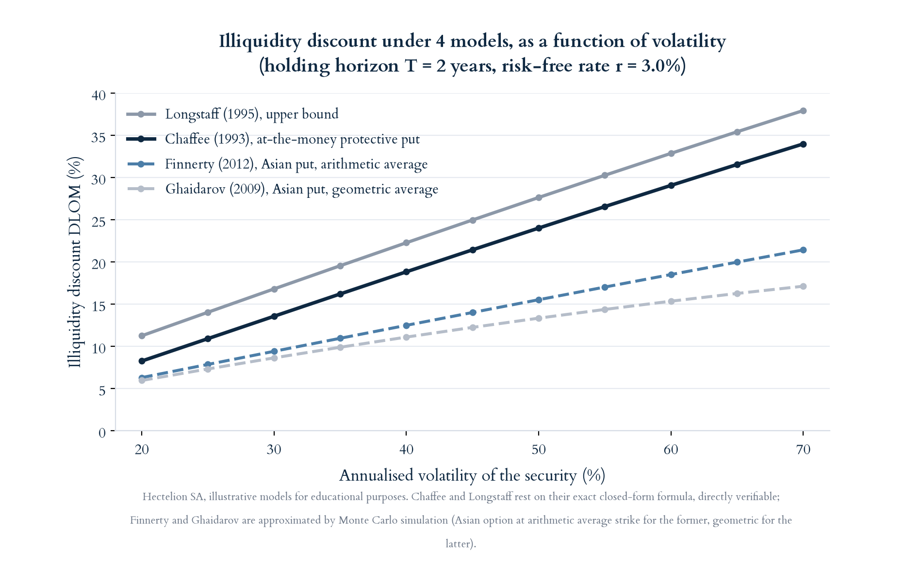
Reading the chart: with horizon and risk-free rate held fixed, all four curves rise with volatility, but at different rates. Longstaff dominates systematically because its theoretical bound is the most conservative; Chaffee sits just below it; Finnerty and Ghaidarov remain markedly lower, with the gap between the four models widening as volatility increases. This is precisely what makes an uncritiqued average across models questionable for a highly volatile security, a point detailed in the Mistakes section below.
When to use the OPM
Using the OPM is warranted as soon as an unlisted company must set the exercise price of new BSPCE or employee stock options after a financing round that introduced a preferred share class, since the value of the common share can no longer be deduced mechanically from the overall valuation announced at the round.
It is also required for the periodic accounting valuation of equity instruments issued as compensation, within the meaning of IFRS 2, when the company publishes consolidated financial statements or is preparing an initial public offering and must retroactively justify the chain of its dilutive-instrument valuations.
A vendor due diligence ahead of a sale transaction, when the capitalisation table includes several successive rounds and several preference ranks, often relies on an OPM allocation to anticipate the actual distribution of sale proceeds among the various shareholders, beyond the single negotiated headline price. A dispute between shareholders over the distribution of exit proceeds, or a challenge by the tax authorities of the exercise price used for an already-issued BSPCE plan, are two other frequent triggers.
Who to call for an OPM allocation
Three criteria distinguish a provider capable of running a defensible OPM allocation. First, genuine technical mastery of option models, Black-Scholes, CRR and Monte Carlo, not just familiarity with their names: the choice of parameters (volatility, horizon) must be argued and benchmarked against observable market references. Second, the ability to precisely map a complex capitalisation table, liquidation ranks, participating clauses, caps, in order to derive the correct breakpoints. Third, independence from the parties involved in the transaction, essential when the result determines a tax exercise price or a distribution among shareholders with potentially diverging interests.
Hectelion carries out this type of engagement as part of its business valuation, startup valuation and financial instrument valuation offerings, with a methodology aligned with IVSC standards and AMF/SIX market practice, and the economic independence of a boutique firm vis-à-vis traditional financial intermediaries. Hectelion is not FINMA-licensed and does not operate on listed transactions; the scope of this article concerns exclusively unlisted companies.
Advantages: rigour, shareholder consistency and auditability
The OPM first brings a rigour that simply dividing total value by the number of shares cannot offer: it explicitly respects the contractual rights of each class, liquidation preference, rank, participating or not, rather than ignoring them. It then ensures shareholder consistency, since the sum of the values allocated to each class always equals, by construction, the total equity value retained upstream, which avoids any arbitrary gap between parties. Finally, it offers valuable auditability: every assumption, volatility, horizon, rate, breakpoint, is explicit and can be discussed, reviewed and benchmarked against market references, which makes it a robust method in the face of a tax audit or an auditor's review.
Limitations: simplifications, sensitivity to assumptions and implementation cost
The main simplification concerns the treatment of employee options: for the sake of clarity, many pedagogical examples, including those in this article, treat BSPCE as fully diluted securities with no strike price of their own, whereas a positive strike price would, strictly speaking, introduce an additional breakpoint and a per-BSPCE value lower than that of the common share until that threshold is crossed.
The result also remains highly sensitive to the volatility and horizon assumptions, two parameters rarely observable directly for an unlisted company and which must be estimated from listed comparables, an unavoidable source of uncertainty that must be documented rather than hidden. Finally, a full implementation, capital mapping, choice of models, cross-checking several calculation methods and several discount models, represents a workload and cost higher than a simple proportional allocation, which is not always proportionate for a very small company with a simple capital structure.
Beyond the divergence between the four illiquidity discount models and the risk of double-counting a synthetic yield q and a full DLOM, already covered in the Mistakes section below, four further methodological limitations of the OPM deserve to be kept in mind:
- A single exit event: the OPM assumes a single horizon T, without modelling an intermediate financing round, dilution, or a partial exit before that date. This simplification is explicitly noted by the AICPA as well as by the IVSC (IVS 200 §130.6), and leads to an imperfect representation of a financing trajectory that, in reality, is marked by several stages.
- A continuous lognormal distribution: the model, visible in the Monte Carlo formula, assumes that the future value of equity follows a smooth lognormal distribution, whereas a young company facing high uncertainty often shows a profile closer to a bimodal distribution, outright success on one side, failure on the other, than a continuous distribution symmetric around a central trend.
- A different form of double-counting, between WACC and volatility: the weighted average cost of capital used upstream to obtain S0, via the DCF or the capitalised earnings value, and the volatility or horizon used downstream in the OPM, can both separately embed a company-specific risk premium. Without care, this premium ends up counted twice, once in the discounting, once again in the implicit risk level of the allocation.
- Unlevering then relevering comparable volatility: the volatility observed on a panel of listed comparables reflects their own financial structure, not that of the unlisted company being valued. Rigorous practice calls for unlevering this volatility to isolate pure operating risk, then relevering it at the actual leverage level of the company being valued, rather than applying a comparable's volatility as-is to a different financial structure.
The 5 mistakes to avoid
Mistake 1: naively dividing the total value by the number of shares
Confusing the value of equity with the value of a common share is the most widespread mistake. As soon as a liquidation preference exists, this division systematically overstates the value of the common share, since it ignores the payment priority enjoyed by senior classes.
Mistake 2: averaging widely divergent DLOM models without question
As the sensitivity chart presented above shows, the gap between Longstaff and Finnerty-Ghaidarov widens sharply as volatility increases. Averaging such divergent models on a highly volatile security, without discussing their respective relevance, amounts to hiding genuine uncertainty behind an arbitrary arithmetic mean.
Mistake 3: ignoring the BSPCE exercise price in the allocation
Treating BSPCE with a positive exercise price as fully diluted common shares without that exercise price overstates their value, since it amounts to granting them a share of value from the very first euro rather than from the threshold at which exercising them actually becomes advantageous.
Mistake 4: combining a synthetic yield q and a full illiquidity discount
Incorporating a positive continuous yield q into the Black-Scholes-Merton model to represent a carry cost, then also applying a full illiquidity discount on top of the result, amounts to counting the same risk twice and artificially undervaluing restricted securities.
Mistake 5: over-weighting the NAV for a fast-growing company
The adjusted net asset value reflects past wealth, not future potential. Giving it a high weight when building the retained value for a fast-growing technology company, whose value rests above all on its future cash flows, biases the total value downward before the OPM allocation even comes into play.
Case 1: Société A, three years after the Series A, valued at €16,644,467
The two cases below concern the same fictitious company, Société A, a French publisher of supervision software for industrial sensors (unlisted), observed at two distinct moments of its development. Its capitalisation table, set at its Series A, does not change between the two cases: 600,000 common shares, 400,000 ADP A preferred shares subscribed at €5.00 per share (i.e. €2,000,000 raised), carrying a non-participating, convertible 1.0x liquidation preference ranking first, and 150,000 BSPCE, for a total of 1,150,000 fully diluted securities. For pedagogical clarity, the BSPCE are treated here as fully diluted securities with no strike price of their own, a simplification discussed in the Limitations section.
Three years after its Series A, Société A has multiplied its recurring revenue by six and is about to close a Series B.
In line with Hectelion's multi-method approach, four market-based approaches are cross-checked: the DCF, trading multiples, transaction multiples, and the capitalised earnings value.
The DCF uses a revenue growth rate of 2%, deliberately conservative for this exercise, and arrives at €9,910,765.
The capitalised earnings value directly capitalises the average adjusted EBITDA of the last three financial years at the WACC, without building multi-year cash flows: Capitalised earnings value = average adjusted EBITDA / WACC. For Société A, average adjusted EBITDA stands at €1,650,000 (€1,150,000, €1,650,000 and €2,150,000 over the last three financial years) and the WACC used is 9.5%, i.e. 1,650,000 / 0.095 = €17,368,421.
These four values are never arbitrarily weighted against one another: such a weighting would give a false sense of precision to an exercise that remains, by nature, an estimate. Hectelion uses here the simple average of the four market-based approaches, an explicit choice rather than a system of weights that cannot be justified term by term.
The adjusted net asset value (adjusted NAV) is calculated separately, and sits outside this average: it starts from book equity (€3,200,000), to which untaxed hidden reserves are added (€1,200,000), net of the corresponding deferred tax at the 25% rate (€300,000), i.e. 3,200,000 + 1,200,000 − 300,000 = €4,100,000.
| Method | Value |
|---|---|
| DCF (2% growth) | €9,910,765 |
| Trading multiples | €19,500,000 |
| Transaction multiples | €19,798,684 |
| Capitalised earnings value (adjusted EBITDA/WACC) | €17,368,421 |
| Retained value (simple average of the 4 market approaches) | €16,644,467 |
| Adjusted net asset value (excluded from the average, floor reference) | €4,100,000 |
The four market-based approaches draw a suggested range of €9,910,765 to €19,798,684, notably wider than a simple range of multiples, with the conservative DCF as the minimum and transaction multiples as the maximum. The adjusted net asset value, even lower than the DCF, confirms its role as a mere floor reference, outside this market range.
This gap between the DCF (€9,910,765) and market multiples (€19.5 to €19.8 million) is not trivial: a deliberately conservative 2% growth rate produces a value almost half that suggested by the market for comparables in the same sector. This is precisely the kind of gap a simple average across several methods is meant to absorb, rather than relying on a single isolated method, whether optimistic or conservative: the same principle that, conversely, forbids over-weighting a patrimonial method such as the NAV for a fast-growing company (Mistake 5 below).
Société A holding a positive net cash position and no significant financial debt as of this date, the net debt bridge is neutral: the values above are already expressed in terms of equity value.
Before any allocation calculation, it should be recalled that the subordination rank between share classes, whether the preference is participating or not, and the conversion ratio never result from a general rule: they stem from the Shareholders' Agreement negotiated between the company and its investors at the time of the financing round.
For this Case 1, the first three parameters are fixed by the agreement signed at the Series A; the last two are specific to the timing of the valuation, not to the agreement itself:
- Liquidation rank: common shares and BSPCE are junior, ADP A is senior with a 1.0x preference.
- Preference type: non-participating (ADP A chooses between receiving its fixed preference OR converting to share pro rata, never both cumulatively, unlike a participating preference which would stack both and reduce the other classes' share accordingly).
- Conversion ratio: 1 ADP A share for 1 common share.
- Liquidity horizon T: 1.5 years, consistent with a Series B seen as close.
- Annualised volatility σ: 38%, estimated from a panel of listed comparables in the industrial software sector.
The ADP A conversion threshold (the second breakpoint) corresponds, by construction, to the point where the per-share value accruing to all securities equals the price paid by investors at the Series A, i.e. €5.00. This threshold equals €2,000,000 / 34.78% = €5,750,000, a figure that depends only on the capital structure and not on the valuation retained at a given point in time.
Liquidation waterfall, Case 1:
| Value tranche | Who receives it | Logic |
|---|---|---|
| €0 to €2,000,000 | ADP A (100%) | Covers the 1.0x non-participating liquidation preference |
| €2,000,000 to €5,750,000 | Common (80%) and BSPCE (20%) of this tranche | ADP A has no incentive to convert, it keeps its fixed preference |
| Above €5,750,000 | All securities pro rata on a fully diluted basis (52.17% common, 34.78% ADP A, 13.04% BSPCE) | Converting becomes more advantageous for ADP A than keeping its fixed preference |
The retained value of €16,644,467 sits far beyond the second breakpoint (a ratio of 2.89x), within the third tranche: ADP A has every economic incentive to convert.
The four calculation methods converge, as expected, to a near-identical result:
| Method | ADP A | Common | BSPCE | Sum (check) |
|---|---|---|---|---|
| Black-Scholes (q=0) | €5,793,748 | €8,680,576 | €2,170,144 | €16,644,467 |
| CRR, N=300 steps | €5,793,713 | €8,680,603 | €2,170,151 | €16,644,467 |
| Monte Carlo, 300,000 draws | €5,794,373 | €8,681,497 | €2,170,374 | €16,646,244 |
| BSM, q=1.5% (alternative) | €5,665,561 | €8,486,870 | €2,121,717 | €16,274,149 |
Black-Scholes and the CRR model coincide to within less than 0.001%; the Monte Carlo simulation deviates by 0.01%, a gap entirely attributable to sampling noise.
The BSM variant with a 1.5% synthetic yield deliberately does not sum to €16,644,467: the missing €370,318 represent the value « absorbed » by the synthetic carry cost over 1.5 years, an alternative that should never be combined with a full illiquidity discount (Mistake 4).
In per-share terms, before the discount, common and ADP A stand at €14.4676 and €14.4844 respectively, a gross gap of only 0.12%: deep in the money, ADP A's liquidation preference protects almost nothing anymore.
The illiquidity discount (σ=38%, T=1.5 years) breaks down as follows across the four models:
- Chaffee (1993): 15.88%
- Longstaff (1995): 18.40%
- Finnerty (2012): 10.46%
- Ghaidarov (2009): 9.52%
- Simple average of the four (retained): 13.56%
This retained average is applied to the gross value of the common share:
€8,680,576 × (1 − 13.56%) = €7,503,056, i.e. €12.5051 per share, against €14.4676 before the discount. This €12.5051 figure is the one that would, in practice, serve as the basis for setting the exercise price of a new BSPCE plan as of this date.
Case 2: Société A, six months after the Series A, valued at €5,200,000
Six months after closing its Series A, Société A shows still-limited traction: first contracts signed, but adjusted EBITDA still negative (−€150,000).
The capitalised earnings value is therefore not calculated at this stage: capitalising a negative EBITDA at the WACC makes no economic sense, and only three market-based approaches are cross-checked.
As in Case 1, Hectelion uses the simple average of the available market-based approaches, with no arbitrary weighting between them.
The adjusted net asset value is calculated separately: it starts from book equity of €875,000, to which untaxed hidden reserves of €300,000 are added, net of deferred tax at the 25% rate (€75,000), i.e. 875,000 + 300,000 − 75,000 = €1,100,000.
| Method | Value |
|---|---|
| DCF | €5,400,000 |
| Trading multiples | €5,400,000 |
| Transaction multiples | €4,800,000 |
| Retained value (simple average of the 3 market approaches) | €5,200,000 |
| Adjusted net asset value (excluded from the average, floor reference) | €1,100,000 |
The three market-based approaches draw a tight suggested range of €4,800,000 to €5,400,000. The adjusted net asset value (€1,100,000), markedly lower, stays outside this market range and serves only as a floor reference.
The company's breakpoints do not change: the ADP A liquidation preference remains at €2,000,000, the conversion threshold remains at €5,750,000, since these thresholds depend only on the capital structure set at the Series A, not on the timing of the valuation.
Liquidation waterfall, Case 2:
| Value tranche | Who receives it | Logic |
|---|---|---|
| €0 to €2,000,000 | ADP A (100%) | Covers the 1.0x non-participating liquidation preference |
| €2,000,000 to €5,750,000 ← retained value sits here | Common (80%) and BSPCE (20%) of this tranche | ADP A has no incentive to convert, it keeps its fixed preference |
| Above €5,750,000 | All securities pro rata on a fully diluted basis | Converting would become more advantageous for ADP A |
Starting assumptions. The liquidation rank, the non-participating nature of the preference and the conversion ratio stay strictly identical to those of Case 1: they come from the same Shareholders' Agreement signed at the Series A, which is not renegotiated between the two cases, a reminder that these parameters are not freely chosen by the valuer but are subject to contractual verification upstream of any such engagement.
- Liquidation rank: unchanged, common and BSPCE junior, ADP A senior with a 1.0x preference.
- Preference type: unchanged, non-participating.
- Conversion ratio: unchanged, 1 ADP A share for 1 common share.
- Liquidity horizon T: 3 years (vs 1.5 in Case 1), the exit being perceived as more distant only six months after the raise.
- Annualised volatility σ: 45% (vs 38% in Case 1), on the same panel of listed comparables, a young company structurally showing more dispersed outcomes than one closer to its Series B.
Unlike Case 1, the retained value of €5,200,000 sits below the second breakpoint (a ratio of 0.90x): it falls within the second tranche.
ADP A has no incentive to convert and captures its fixed €2,000,000 preference first; common and BSPCE share only the remaining €3,200,000.
| Method | ADP A | Common | BSPCE | Sum (check) |
|---|---|---|---|---|
| Black-Scholes (q=0) | €2,274,760 | €2,340,192 | €585,048 | €5,200,000 |
| CRR, N=300 steps | €2,274,516 | €2,340,387 | €585,097 | €5,200,000 |
| Monte Carlo, 300,000 draws | €2,275,104 | €2,341,287 | €585,322 | €5,201,713 |
In per-share terms, before the discount, ADP A stands at €5.6869 against €3.9003 for common and BSPCE, a gross gap of 45.81%, more than a thousand times larger than in Case 1.
Proximity to the conversion threshold radically changes the distribution of value across classes, even though total equity value (€5,200,000) represents only 27% of that in Case 1.
The volatility used is higher than in Case 1 (45% versus 38%), consistent with the earlier, less proven stage of the company, and the horizon T is longer (3 years versus 1.5), the exit being less imminent.
The illiquidity discount is mechanically higher as a result:
- Chaffee (1993): 24.90%
- Longstaff (1995): 30.33%
- Finnerty (2012): 17.35%
- Ghaidarov (2009): 14.67%
- Simple average of the four (retained): 21.81%
Applied to the gross value of the common share: €2,340,192 × (1 − 21.81%) = €1,829,745, i.e. €3.0496 per share.
The comparison of the two cases is the central pedagogical point of this article: the same capital structure, the same contractual rights, produce a gap between classes of 0.12% three years after the raise, against 45.81% six months after. It is not the liquidation preference that changes, it is the position of total value relative to the conversion threshold.
Word from the CEO
« The OPM has the particular merit of forcing what a simple division by the number of shares leaves implicit to become explicit: who gets paid first, and above what threshold everyone truly benefits from growth. It is as much a discipline of transparency as it is a calculation tool. »
« Case 2 of this article illustrates a point many executives underestimate: six months after a raise, the value gap between a common share and a preferred share can exceed 40 or 50%, simply because the company has not yet created enough value above the price paid by its investors. Setting a BSPCE exercise price without accounting for this exposes the company to a very real requalification risk. »
« At Hectelion, we always cross-check several OPM calculation methods and several illiquidity discount models, not out of excessive caution, but because the convergence or divergence of results is itself useful information for the executive and their shareholders. »
Aristide Ruot, Ph.D.
Founder | Chief Executive Officer, Hectelion SA
FAQ: the 10 essential questions on the OPM and the illiquidity discount
Introduction: what to remember before the questions
This FAQ gathers, in short form, the points most frequently raised by executives, CFOs and investors encountering an OPM allocation for the first time.
Q1: What is the OPM in business valuation?
The OPM is a method that models each class of securities of an unlisted company as an option on the total equity value, in order to allocate that value across classes according to their respective rights.
Q2: Why not simply divide the total value by the number of shares?
Because that division assumes all shares carry identical rights, which is only true in the absence of any liquidation preference. As soon as a senior class exists, this method systematically overstates the value of common shares.
Q3: What is the difference between Black-Scholes and Black-Scholes-Merton in this context?
Black-Scholes-Merton adds a continuous yield q, traditionally a dividend, but which can also be used as a proxy for the carry cost of an illiquid security. Absent any dividend and with q at zero, the two formulas coincide exactly.
Q4: Why use four calculation methods if they converge to the same result?
Precisely because they converge: the agreement between Black-Scholes, CRR and Monte Carlo acts as a consistency check on the calculation. A significant divergence between these methods would signal a parameterisation error.
Q5: What is a breakpoint in the context of the OPM?
A breakpoint is a total value level beyond which the economic behaviour of at least one share class changes, most often the threshold at which a preferred share becomes more advantageous converted than keeping its fixed preference.
Q6: How should the volatility and holding horizon (T) be chosen?
Volatility is generally estimated from a panel of listed comparables in the same sector. The horizon T corresponds to the expected duration until the most likely liquidity event, exit, IPO or major new round, and must be documented and justified.
Q7: Why four different illiquidity discount models, and which one should be chosen?
Each model rests on a different behavioural assumption about what a restricted holder « loses ». In practice, retaining an average or a range across several models, documented and justified, is preferable to a single undiscussed choice.
Q8: Does the illiquidity discount apply to all share classes?
In the two cases presented in this article, the discount was applied only to the common share, consistent with common practice when the objective is to set a BSPCE exercise price. A fuller analysis may, however, justify a discount specific to each class, depending on the relative liquidity of each.
Q9: When is the OPM not the right method?
When the company expects a very short-term and identifiable liquidity event, a current value method (direct waterfall allocation) may suffice. When several distinct, probability-weighted exit scenarios exist (an IPO in two years, an acquisition in one year, for example), a PWERM approach, which weighs discrete scenarios rather than a continuous distribution, is often more appropriate.
Q10: What is the link between the OPM and setting the BSPCE exercise price?
The per-common-share value obtained from the OPM allocation, net of the illiquidity discount, serves directly as the reference for setting the exercise price of a new BSPCE plan as of the valuation date, as illustrated in Cases 1 and 2 above.
Estimate the value of your company with Acontos, Hectelion's online simulator
To extend this reading with a concrete figure, Hectelion provides Acontos, its online audit, due diligence and business valuation tool. Powered by Claude Sonnet 5 by Anthropic and calibrated on Hectelion's methodology, it reads your financial statements, normalises EBITDA, applies real sector multiples and rebuilds a net debt bridge to estimate the value of your shares within minutes. Launch the free valuation simulator: the tool is confidential, retains no document, and does not replace a formal OPM allocation for a company with several share classes, but it gives a first reliable order of magnitude of your total equity value before discussing it with our teams.
Conclusion: a demanding method, but the only one that respects each class's rights
The OPM is not a valuation method among others: it only comes into play once a total equity value has already been determined through DCF, multiples or NAV, in order to correctly allocate it across share classes with unequal rights. It is this distinction, between valuing and allocating, that explains why a common share is almost never worth the result of a simple division.
The two worked cases in this article, built on the same fictitious company observed at two moments of its life, show just how much this allocation can vary: a 0.12% gap between classes three years after a raise, a 45.81% gap six months after the same raise. Between the two, nothing changed in the contractual rights: only the position of total value relative to the preference's conversion threshold shifted.
The convergence of the four calculation methods, Black-Scholes, Black-Scholes-Merton, CRR and Monte Carlo, is reassuring as to the technical robustness of the result. The divergence, by contrast, of the four illiquidity discount models, Chaffee, Longstaff, Finnerty and Ghaidarov, is a reminder that a degree of documented judgement remains unavoidable, and must be owned explicitly rather than hidden behind a single figure.
Summary of the article
The OPM models each share class as an option on total equity value, in order to allocate that value, previously determined through DCF, multiples and NAV, across common shares, preferred shares and BSPCE according to their respective contractual rights.
Four methods allow this allocation to be calculated, Black-Scholes, Black-Scholes-Merton, the Cox-Ross-Rubinstein binomial tree and Monte Carlo simulation, all of which converge to a very close result for identical assumptions.
The illiquidity discount then applied to restricted securities rests on four models with different logics, Chaffee and its at-the-money protective put, Longstaff and its lookback-option upper bound, Finnerty and its average-strike Asian put, Ghaidarov and his correction, whose results can vary by a factor of two depending on the volatility used.
The two worked cases of Société A illustrate the central point of this article: the proximity of total value to a liquidation preference's conversion threshold determines, far more than the contractual rights themselves, the magnitude of the value gap between share classes.
Sources
- American Institute of CPAs (AICPA), Accounting and Valuation Guide, Valuation of Privately-Held-Company Equity Securities Issued as Compensation
- Black F. and Scholes M. (1973), The Pricing of Options and Corporate Liabilities, Journal of Political Economy, vol. 81, no. 3
- Chaffe D.B.H. III (1993), Option Pricing as a Proxy for Discount for Lack of Marketability in Private Company Valuations, Business Valuation Review, vol. 12, no. 4
- Cox J.C., Ross S.A. and Rubinstein M. (1979), Option Pricing: A Simplified Approach, Journal of Financial Economics, vol. 7, no. 3
- Damodaran A., New York University Stern School of Business, work on real options and the illiquidity discount
- Finnerty J.D. (2012), An Average-Strike Put Option Model of the Marketability Discount, The Journal of Derivatives, vol. 19, no. 4
- Ghaidarov S. (2009), Analysis and Critique of the Average Strike Put Option Marketability Discount Model, SSRN Working Paper
- Internal Revenue Service (IRS), Discount for Lack of Marketability Job Aid for IRS Valuation Professionals
- International Valuation Standards Council (IVSC), IVS 200, Business Valuation, §130.5-130.8
- Longstaff F.A. (1995), How Much Can Marketability Affect Security Values?, The Journal of Finance, vol. 50, no. 5
- Merton R.C. (1973), Theory of Rational Option Pricing, Bell Journal of Economics and Management Science, vol. 4, no. 1
Author
Aristide Ruot, Ph.D.
Founder | Chief Executive Officer, Hectelion SA